
Giemsa-staining Method
Biodosimetry of human exposure to radiation: A manual for detecting stable chromosome aberrations by the conventional Giemsa staining method
Akio A. Awa
Former Chief of Genetics Department, Radiation Effects Research Foundation, Hiroshima
Contents
- Introduction
- Preparation of metaphases
- Selection of metaphases
- Nomenclatures for describing aberrations
- Characteristics of chromosome groups (karyotyping)
- Normal variation of chromosomes
- Stable aberrations – introduction
- Stable aberrations – deletion
- Stable aberrations – inversion
- Stable aberrations – reciprocal translocation
- Example of misinterpretation
- Conclusions
1. Introduction
The frequency of chromosome aberrations in blood lymphocytes has been used to estimate radiation doses received by individuals. There are two kinds of aberrations, stable and unstable.
Unstable aberrations, represented by dicentrics and centric rings, are easily detected, but they are lost with time following cell divisions. Thus, as years pass following radiation exposure, the frequency declines, and these aberrations are not useful for dose estimation. In contrast, stable aberrations, represented by reciprocal translocations and pericentric inversions (i.e., inversions that include centromeres), are not affected by cell division and hence do not disappear with time. However, these aberrations have their own problem: they are difficult to identify by the conventional method and hence the detection efficiency has remained low.
We started to examine chromosome aberration frequencies of atomic-bomb survivors in the late 1960s, but unstable aberrations had mostly disappeared by that time. Hence, detection of stable aberrations was the only choice. Only the conventional Giemsa staining method was available in those days, so we worked to establish a laboratory manual and continued the work for nearly 30 years.
Recently, a new chromosome painting technique (FISH) has become available to replace conventional Giemsa staining. This new technique uses painting of specific chromosomes with fluorescent dyes through in situ hybridization and enables chromosomal exchanges between the painted and non-painted chromosomes to be detected objectively. When we compared the results of the two methods for the same 200 survivors, we found that the conventional method detected translocations with nearly 70% of that by FISH (Nakano M et al. Int J Radiat Biol 77:971-7, 2001).
We felt recently that too much emphasis is given to FISH, as if no other methods can detect stable aberrations, which is not true for us. For this reason we decided to open this manual to the public so that scientists working in this field may understand that there are different methods to detect stable aberrations.
Although FISH has many technical advantages, the costs of performing FISH and installing the ultraviolet microscope are high. Thus, we sought to provide information that the conventional Giemsa staining can also detect a fairly good fraction of stable aberrations if one is well familiar with human karyotypes.
2. Preparation of metaphases
This manual has been prepared for those who experienced in cytogenetics, so I thus omitted technical procedures for preparing metaphases. Please refer to published manuals for this purpose. For example, refer to
Verma RS and Babu A: Human chromosomes. Manual of basic techniques. New York, Pergamonn Press, 1989.
3. Selection of metaphases
In Giemsa staining, we use a green or yellow filter that provides the best contrast for observing by eye and photography.
When we select the metaphases, we first use low-magnification lenses. There is one basic rule, specifically, not all metaphases that are apparently suitable under low magnification are actually suitable for analysis. (Low magnification implies 10 (eye lens) × 10 (objective lens) = ×100 or 10 × 20 = ×200 magnification; high magnification implies 10 (or 15) × 100 (oil objective or dry lens) = ×1000 (or 1500). Whenever the metaphases selected under low-power magnification are suspicious, moderate magnification, such as ×400 (10 × 40), is recommended for confirmation.
The conditions of metaphases suitable for analysis are as follows:
- The 46 chromosomes distribute evenly on the slide in a circular or slightly elliptical shape.
- Ideally, chromosomes should not overlap, although some overlap is allowed.
- Centromeres should be observed in all chromosomes. When chromosomes overlap, centromeric portions should not overlap.
- Chromosomes should be stained evenly. In other words, all the chromosomes should have the same staining density. A chromosome on the edge of the microscopic field with darker or lighter staining should be excluded. This is due to a torsional stress during the air-drying process that may cause differences in chromosome length even between homologous chromosomes. Generally, lighter (darker) staining results in longer (shorter) chromosomes.
- The total number of chromosomes should be 46, but chromosomes are difficult to count under low magnification. The possible variation should be 46 ± 1.
- Sister chromatids comprising each chromosome should be clearly seen.
- Avoid metaphases with heavily condensed chromosomes (too much effect of colcemid) or with visible chromatin spiral. In both cases, centromere positions are not clearly seen.
Of these seven conditions, only (1) may be met under low magnification; the remaining conditions should be met primarily under moderate to high magnification. Let us now consider the examples in Figures 1 to 3. All of these metaphase pictures were taken under ×1000 (10 × 100) magnification.
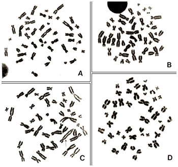
Figure 1
Figures 1 A to D represent good metaphases for analyses. Chromosomes in Figure 1A are well spread with no overlaps. In contrast, chromosomes in Figures 1B and 1D tend to be shorter, which indicates that the cells are at a late stage of metaphase and that the effect of colcemid was slightly too strong. Chromosomes in Figure 1C also appear good, but, as indicated by the dotted arrow, two chromosomes are attached end-to-end and appear as if they constitute one abnormal chromosome (a dicentric chromosome).
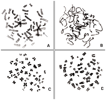
Figure 2
Examples of unsuitable metaphases are shown in Figures 2 and 3. In Figure 2A, there are too many overlapping chromosomes including centromere regions, so it is impossible to identify centromere positions and, hence, karyotyping cannot be achieved. Chromosomes in Figure 2B are not in metaphase but rather in prophase, and individual chromosomes cannot be identified. Figures 2C and 2D represent chromosomes that are too condensed so that centromere positions are not clear. Some chromosomes in Figure 2D are folded, and their lengths cannot be properly measured.
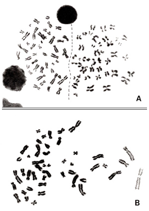
Figure 3
Figure 3A represents two metaphases located side by side. In this picture, the borderline between the two cells can be easily seen because the stage of chromosome condensation is different (dotted line). However, one should keep in mind that two daughter cells may occasionally begin the second mitosis simultaneously when located side by side on the slide. In such cases, conditions of chromosome condensation are very similar in both cells. Hence, the borderline between the two cells cannot be seen clearly. Under such circumstances, the two cells may exchange some chromosome, and one may easily score aberrations that are artifacts.
Figure 3B represents an example of different condensation among chromosomes in one cell. Chromosomes on the left are darkly stained whereas the staining becomes lighter toward the right. Such a metaphase should be avoided as the extended chromosomes may be interpreted as aberrations.
The metaphases selected under low magnification will be used for karyotyping under high magnification. The procedures are as follows.
- Score the number of chromosomes. In the beginning, you may use a counter for this purpose, but you will soon be able to count 46 chromosomes in your mind. The total number of chromosomes must be 45, 46, or 47.
- Examine the shape and length of each chromosome (karyotyping). Usually, we take microscopic photographs at 2000- to 3000-fold magnification, cut out each chromosome, and arrange the chromosomes in order with their homologues to find an abnormality.
- As the procedure is very time consuming, we need to train ourselves to examine chromosomes under the microscope. If you can achieve it, you will no longer need to take photographs of normal cells and cut out each chromosome but only take photographs of metaphases with suspected or definitive abnormalities. However, it is very important to take photographs of any metaphases with suspected aberrations.
4. Nomenclature for describing aberrations
You are probably familiar with the characteristics of the 46 human chromosomes. The rules are described in ISCN (An International System for Human Cytogenetic Nomenclature), and it is necessary to follow these rules when describing an aberration. These rules contain lists of abbreviations describing chromosomes, chromosome segments, and aberrations. I have listed in Table 1 some of these that I felt important.
|
Table 1. Major symbols to describe stable aberrations
|
||
|
| cen | centromere |
| cx | complex interchange |
| del | deletion |
| h | heterochromatin |
| ins | insertion |
| inv | inversion |
| mar | marker chromosome |
| – | loss |
| p | short arm of chromosome |
| pcd | premature centromere division |
| + | gain |
| q | long arm of chromosome |
| rcp | reciprocal |
| s | satellite |
| ; | To separate altered chromosomes and breakpoints |
| t | translocation |
Before starting metaphase examination, I will describe some fundamental nomenclature.
Each chromosome bears a constriction called a centromere (“cen,” Table 1) and is divided into two parts by the centromere, a longer part termed long arm (q) and shorter part termed short arm (p). For karyotyping, we place short arms above the long arms.
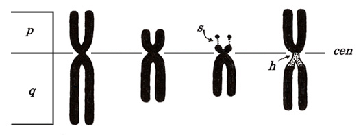
Figure 4
As shown in Figure 4, some chromosomes have snail-eye-like structures at the end of their short arms. These are termed satellite (“s”) and are located at chromosomes 13, 14, 15, 21, and 22. Ribosomal RNA genes are located there.
The structure indicated with “h” means a secondary constriction. The first constriction means a centromere, which exists in every chromosome. Instead, “h” appears only in chromosomes 1, 9, and 16, near the centromere, and is thin and lightly stained (heterochromatin). The Y chromosome has “h” at the end of a long arm but not in the centromeric region.
To understand each chromosome, see Table 2. The Centromere Index (CI) stands for the ratio (percentage) of short arm length to the whole length of a chromosome. If CI is closer to 50, this means that the centromere is located in the middle of the chromosome; if the CI is small, this means that the centromere is located terminally.
|
Table 2. Chromosome relative lengths (percent of total autosomes*) and and Centromere Index (CI)**
|
|||
|
|
1
|
9.11 ( 4.43 : 4.68 ) | 48.6 |
|
2
|
8.61 ( 3.35 : 5.26 ) | 38.9 |
|
3
|
6.97 ( 3.30 : 3.67 ) | 47.3 |
|
4
|
6.49 ( 1.80 : 4.69 ) | 27.8 |
|
5
|
6.21 ( 1.66 : 4.55 ) | 26.8 |
|
6
|
6.07 ( 2.30 : 3.77 ) | 37.9 |
|
7
|
5.43 ( 2.01 : 3.42 ) | 37.0 |
|
X
|
5.16 ( 1.94 : 3.22 ) | 37.5 |
|
8
|
4.94 ( 1.62 : 3.32 ) | 32.8 |
|
9
|
4.78 ( 1.56 : 3.22 ) | 32.7 |
|
10
|
4.80 ( 1.55 : 3.25 ) | 32.3 |
|
11
|
4.82 ( 1.95 : 2.87 ) | 40.5 |
|
12
|
4.50 ( 1.23 : 3.27 ) | 27.4 |
|
13
|
3.87 ( 0.64 : 3.23 ) | 16.6 |
|
14
|
3.74 ( 0.69 : 3.05 ) | 18.4 |
|
15
|
3.30 ( 0.58 : 2.72 ) | 17.6 |
|
16
|
3.14 ( 1.33 : 1.81 ) | 42.5 |
|
17
|
2.97 ( 0.94 : 2.03 ) | 31.9 |
|
18
|
2.78 ( 0.74 : 2.04 ) | 26.6 |
|
19
|
2.46 ( 1.10 : 1.36 ) | 44.9 |
|
20
|
2.25 ( 1.03 : 1.22 ) | 45.6 |
|
21
|
1.70 ( 0.49 : 1.21 ) | 28.6 |
|
22
|
1.80 ( 0.51 : 1.29 ) | 28.2 |
|
Y
|
2.21 ( 0.51 : 1.70 ) | 23.1 |
| *Percentage of each chromosome to a total of 22 pairs of autosomes. **CI = (short arm length ÷ [short arm length + long arm length]) × 100. |
5. Characteristics of chromosome groups: Karyotyping
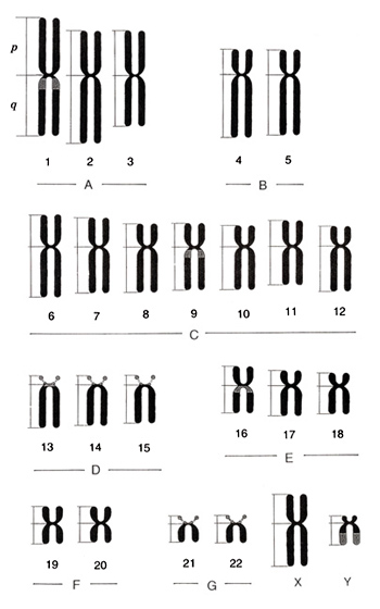
Figure 5
The rule of karyotyping is to arrange 22 autosomes following the size and sex chromosomes, X and Y, at the end. Chromosomes are classified into seven groups, A to G, by the length and centromere position. Characteristics of each chromosome group will be explained below.
Figure 5 shows an ideogram or idiogram of human chromosomes, and Figure 6, metaphases and karyotypes of a male and a female. They may help you to understand the characteristics that I am going to describe. The information shown in Table 2 was taken from ISCN (1985), but I omitted standard deviations (on the order of 5 to 10%) associated with the observation. Because group-C chromosomes are the most difficult to identify, I will explain them at the end.
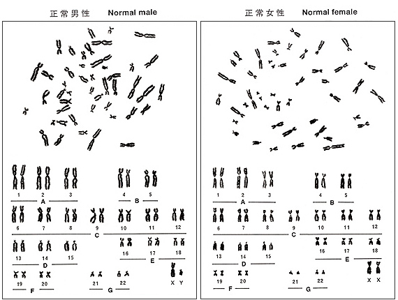
Figure 6
Group A (chromosomes 1 to 3)
This group is comprised of the three largest pairs of chromosomes with centromeres located in the middle regions. Chromosomes 1 and 2 have similar lengths, but their centromere positions are different. Chromosome 1 has its centromere in the middle, while it is slightly shifted toward the short arm (or CI = 40%) in chromosome 2. Chromosome 1 bears a secondary constriction, an “h”, and can be easily distinguished from chromosome 2. Chromosome 3 has a centromere in the middle and is shaped similarly to chromosome 1 (CI = 48.6% in chromosome 1 and CI = 47.3% in chromosome 3), but chromosome 3 is about 20% shorter than chromosome 1. Thus, chromosome 3 can be easily distinguished with experience.
One possible problem is “h” in chromosome 1 because there are individual variations. Some may carry an “h” in both number 1 chromosomes, in only one number 1 chromosome, or in neither number 1 chromosome. The “h” is located at the upper portion of the long arm immediately below the centromere, like a round shoulder below a long neck of a stork (a long-necked bird). Please refer to chromosome 1 on the right in Figure 6 (left). As the heterochromatin content increases, the “h” region becomes longer. This is not regarded as a structural abnormality but is called a normal variant or heteromorphic chromosome. If one of the two parents bears the chromosome, one half of the progeny inherits the chromosome according to the Mendelian law.
Group B (chromosomes 4 and 5)
Group B is comprised of two pairs of large chromosomes with centromeres in the sub-terminal regions. Group B chromosomes are the second longest (about 75% of group A chromosomes) and CI = 27 to 28%, or the short arm comprises nearly one-fourth of the chromosome. The long arm is nearly the same as the long arm of chromosome 1. Number 4 and number 5 chromosomes are very similar, so it is not possible to distinguish them by the conventional method.
Group C (to be described later)
Group D (chromosomes 13 to 15)
Group D is comprised of three pairs of middle-sized chromosomes with centromeres located terminally (CI = 17-18%). The whole chromosome length corresponds to the short arm of chromosome 3. All of these chromosomes bear an “s” (satellite). These chromosomes are rather easy to distinguish.
The “s” may not be visible in every cell. Satellites of group-D and group-G chromosomes form a focus, termed satellite association, which is the site for ribosomal RNA synthesis.
As with the “h” of chromosome 1 (heteromorphic chromosome), the shape and size of the “s”‘s are known to vary with individuals, and the variation is genetically determined. Deletion of “s”‘s is also observed in rare cases but does not relate to any hereditary diseases.
Group E (chromosomes 16 to 18)
Group E is comprised of three pairs of chromosomes that are slightly smaller than group-D chromosomes. Chromosome 16 has the centromere near the middle (CI = 42%), whereas chromosomes 17 and 18 have centromeres in more distal regions (CI = 32% and 27%, respectively). Hence, their p-arms tend to be clearly shorter than that of chromosome 16. Chromosomes 17 and 18 are very similar but can be distinguished with experience since the short arm of chromosome 18 is slightly shorter than that of chromosome 17.
Chromosome 16 has an “h” as does chromosome 1 and considerable variation exists in its size and shape.
Group F (chromosomes 19 to 20)
Group F is comprised of two pairs of short chromosomes with their centromeres located in the middle regions. Chromosomes 19 and 20 cannot be distinguished.
Group G (chromosomes 21, 22, and Y)
Group G is comprised of the smallest two pairs of autosomes with an “s” at the end of every short arm. As the Y chromosome belongs to this group, the total number is five in males and four in females, but the Y chromosome does not contain an “s”. Although chromosome 21 was found later to be smaller than chromosome 20, the original chromosome order was kept in karyograms.
The Y chromosome belongs to this group and is slightly longer than chromosomes 21 and 22. As the lower half of q-arm is heterochromatic, the Y chromosome has a normal variation in its total length. It is easy to distinguish it from other group-G chromosomes by it lack of “s” and presence of “h” that is stained lighter, and the sister chromatids of “h” tend to be attached.
Group C (chromosomes 6 to 12, and X)
Group C is composed of middle-sized chromosomes, comprising sevem pairs of autosomes and one or two X chromosomes. Thus, males carry a total of 15 group-C chromosomes, and females carry 16. Centromeres are located either in the middle or sub-terminal regions. The X chromosome is one of the large chromosomes in this group. Because every group-C chromosome looks similar, chromosomes of this group are the most difficult to distinguish. Nonetheless, I will try to describe the basic characteristics.
When chromosomes of this group are arranged in order, you may find differences in centromere positions. Specifically, CIs are large for chromosomes 6, 7, 11, and X; slightly smaller for chromosome 9; and smaller for chromosomes 8, 10, and 12. In other words, the trend of centromere position from chromosomes 6 to 12 is large – large – small – slightly small (with “h”) – small – large – small, and is actually bumpy.
Chromosome 6 is the largest among the group-C chromosomes, and you will recognize it is larger than chromosome 7 if you put the chromosomes in order. However, it will take some time to recognize the small difference between the two chromosomes under the microscope (i.e., without arranging the chromosomes in order). Quite often, the middle part of chromosome 6p is lightly stained.
Chromosomes 7 and X are almost impossible to distinguish. Thus, the three (in males) or four (in females) second largest chromosomes after chromosome 6 with large CI’s are regarded as chromosomes 7 and X.
I should mention here that cells from women aged over 50 years occasionally show one of the two X chromosomes with no centromeric constriction, and the chromosome looks like one large acentric fragment. These chromosomes are termed “premature centromere division (PCD)” chromosomes and represent one inactive X chromosome in female cells. The frequency tends to increase with donor age.
Chromosomes 8, 10, and 12 show centromeres at slightly higher positions; no other unique characteristics are present. Chromosomes 10 and 12 look very similar and are difficult to distinguish. In practice, the smallest pair of chromosomes is assigned as chromosome 12.
Chromosome 9 may be distinguished from other group C chromosomes with relative ease. This is because it carries a secondary constriction, an “h”, as do chromosomes 1 and 16 with individual variations. As mentioned earlier, if we consider the centromere as a head of a stork, the “h” corresponds to a round shoulder toward the wings. Such a variation is observed in families with varying frequencies.
Chromosome 9 also shows pericentric inversion at a frequency of about 1% in a population. In this case, 100% of the metaphases should show the same characteristics. The inversion does not accompany any clinical abnormalities, and, hence, this is regarded as one of the normal variations.
These are the characteristics of each group. The basic attitude to train yourself is to enumerate the exact number of chromosomes for each group, namely, females should have A = 6, B = 4, C = 16, D = 6, E = 6, F = 4, and G = 4 and males should have A = 6, B = 4, C = 15, D = 6, E = 6, F = 4, and G = 5. This approach can also tell you the gender of the blood samples.
In summary, if you don’t find anything wrong in the number of chromosomes in each group, you may consider the cell is normal. However, if the number is increased in one group and decreased in another group, an aberration may be present.
Although I attempted to describe chromosomes from groups A to G here, you don’t need to follow this order. I personally start with groups D and G, followed by F, E (chromosomes 16, and 17 plus 18), A, B, and C at the end but most carefully.
I would recommend drawing metaphase sketches. Although it might take some time at the beginning, I assure you that you can do it very quickly after some experience. Drawing sketches is useful as proof of the aberrations.
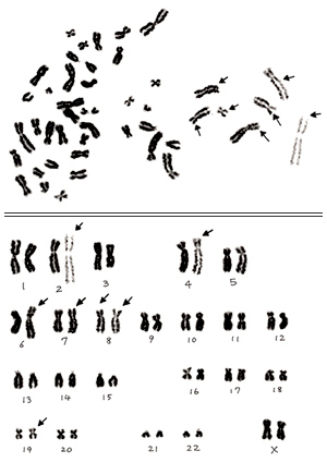
Figure 7
In section 3, I presented one example of an inappropriate metaphase that showed partial distortion (Figure 3B). As you see in the karyogram shown in Figure 7, several chromosomes at the right are abnormally extended, as even spiral structure can be seen. Those marked by arrows are especially extended compared with their homologues. I judge this is a normal cell, but I should say that you must discard this metaphase before starting karyotyping.
6. Normal variation of chromosomes
Here I will explain the normal variation of chromosomes that was briefly explained in the previous section. As these variations appear in every cell, we may easily distinguish these normal variations from radiation-induced aberrations.
In human populations, there are individuals bearing chromosomal variations at frequencies of 2% to 5%. These are mostly related to “h”‘s and “s”‘s, and I have already explained some of these previously. Karyotypes of two examples are shown in Figures 8 and 9.
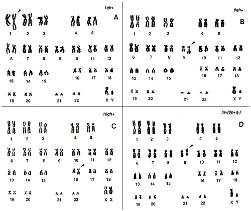
Figure 8
Figure 8A shows a long, extended chromosome 1; Figure 8B, a long chromosome 9; and Figure 8C, a long chromosome 16. All of these show an extended “h” and may be regarded as abnormal if one sees only one metaphase from the individuals. In particular, chromosome 16 requires caution because it cannot be distinguished from a group-C chromosome (number 10 or 12) unless one pays attention to the “stork’s neck”.
Figure 8D represents the inversion of chromosome 9. This is an inherited characteristic with no symptoms and appears at a frequency of nearly 1% in a population.
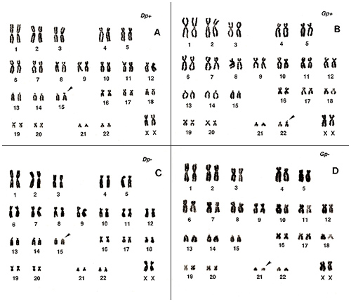
Figure 9
Figure 9 shows the normal variation in the short arms or “s”‘s of group-D and group-G chromosomes. Both gain (Figure 9A, one group-D chromosome; Figure 9B, one group-G chromosome) and loss (Figure 9C, one group-D chromosome; Figure 9D, one group-G chromosome) exist. As these changes are clear, recognition is easy.
7. Stable aberrations – Introduction
The basic approach for detecting stable aberrations is to use chromosome length, CI, “h,” and “s” to objectively find subtle differences between normal and abnormal cells.
Let us think of the length. Although the alteration of length may be the same, its detection rate depends on whether it happened in a large or a small chromosome. For example, an increase from 8 µm to 10 µm (25% increase) of a chromosome cannot be firmly established, but the same 2 µm increase in a small chromosome should be easily detected.
Let us take another example. When one homologue is 10% longer than its counterpart, there are two possibilities: both short and long arms are equally extended with no change in CI, or one of the two arms is extended with an altered CI. The first case is a normal variation, but the second is probably an aberration. This means that both different length and altered CI are good indicators for recognizing an aberration.
In addition to absolute length and CI value, the detection probability is also affected by stage differences in metaphase (early or late metaphase), thickness of the chromosome, or darkness of staining. Darkly stained chromosomes tend to be shorter, and pale ones, to be longer. In other words, it is generally true that chromosome mass, i.e., darkness (or thickness) × length, is constant.
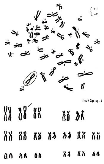
Figure 10
Let’s move to examples for detecting stable aberrations. Figure 10 (upper panel) shows various marks near the centromeres. Numbers 1, 2, 3, 16, 17, and 18 indicate chromosome numbers, and B, D, F, and G represent chromosome groups. Group-C chromosomes are marked with small circles, and Y indicates the Y chromosome. You will soon understand that identifying the Y chromosome is one of the easiest tasks.
Chromosomes of Y, group G, group D, numbers 16, 17, and 18 are normal. There are four group-B chromosomes and 15 group-C chromosomes, and they look normal. In group-A chromosomes, number 3 chromosomes are normal, but there are three number 1 chromosomes and only one number 2 chromosome as indicated by +1 and -2 on the top right. One of the three apparent number 1 chromosomes was marked by a circle because it did not carry an “h” next to the centromere.
In this metaphase, only one chromosome looks abnormal; the remaining chromosomes look normal. As shown in the karyotype (Figure 10 (lower panel)), the aberration was assigned as inv(2p+q-). When only one chromosome looks abnormal, either a deletion or an inversion is suspected.
8. Stable aberrations – deletion
Deletion is an abnormality with a shortened chromosome arm of one chromosome. As deletion affects only one chromosome, it is difficult to distinguish from an inversion. Deletion more often occurs in large chromosomes. Four examples are shown in Figures 11 and 12, in which the group-A or group-B chromosome is affected. If deletion happens in small chromosomes, a subtle change may be detected easily. The detection rate is thus likely to be inversely related to the chromosome length.
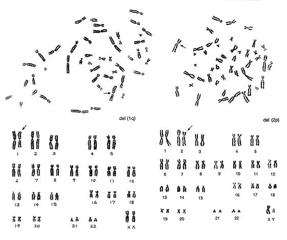
Figure 11
Figure 11 (left) shows no abnormalities for chromosomes of group B to G, while something is wrong in group-A chromosomes. There is only one number 1 chromosome but three number 3 chromosomes. Thus, we would expect del(1q). The metaphase shown in Figure 11 (right) lacks one chromosome 2 but has one abnormal chromosome that looks like a group-B chromosome. As both arms are slightly longer than those of normal group-B chromosomes whereas the long arm length is nearly equal to that of chromosome 2q, we assigned the aberration as del(2p).
Figure 12 shows two abnormal metaphases that are rather difficult to detect. Both involve one group-B chromosome. On the left figure, one group-B chromosome indicated by an arrow seems to be abnormal as its short arm length is shorter than those of the other three group-B chromosomes. As the long arm length looks normal, we judged it as del(Bp). However, if the long arm length of the abnormal chromosome were longer than those of the remaining three group-B chromosomes, then we would have suspected an inversion. The critical information is whether CI is 20% or less.
Figure 12 (right) also involves an aberration in one group-B chromosome. One of the four group-B chromosomes looks very similar to a small group-C chromosome. The karyoptype shows one additional group-C chromosome with a deficiency of one group-B chromosome. We judged it as del(Bq).
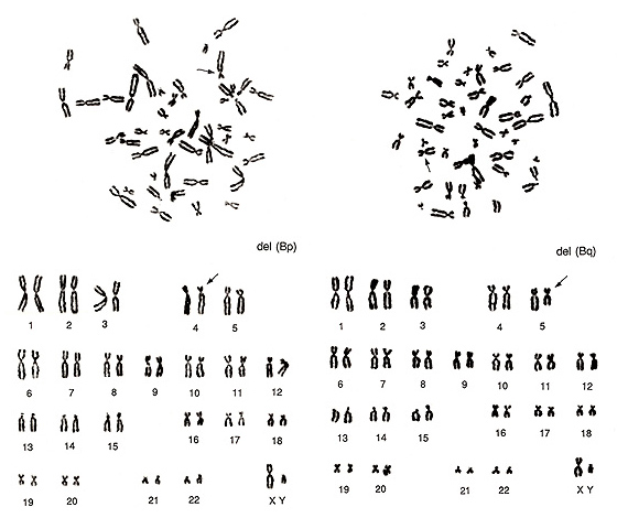
Figure 12
The key point for identifying a deletion is that only one chromosome of one group is affected. This may result in two ways: either creation of one marker chromosome not belonging to any known groups along with lack of one chromosome from one group, or one additional chromosome in the smaller group (i.e., deletion of one chromosome B may result in addition of one group-C-like chromosome).
9. Stable aberrations – inversion
The distinguishing characteristic of inversion is creation of one abnormal chromosome not belonging to any known group and a consequent loss of one chromosome from one group. Such an abnormal chromosome is called “a marker chromosome” and is observed in cases of deletion, inversion, and translocation. In inversion, the total chromosome length remains within the normal range but CI is altered. Thus, there is no chromosome with altered length in each group.
Inversions are not detectable if the two breakpoints on the two arms are located either at nearly the same distances from the centromere or at nearly the same distances from each end of the two arms.
Figure 13 shows two inversions of chromosome 2 indicated by arrows.
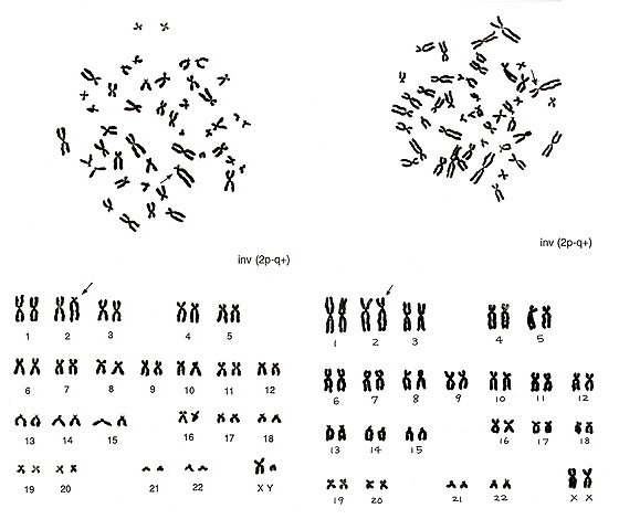
Figure 13
The abnormality at left is easy to find because the shape of the inverted chromosome is unique. As the remaining chromosomes are normal, inv(2) is obvious. The figure at right shows another inverted chromosome 2 in which the p arm is slightly shorter and the q arm is slightly longer while the total length remains normal. CI is altered. Both inversions are described as inv(2p-2q+).
Figure 14 (left) includes one inversion of a group-B chromosome, and Figure 14 (right), one inversion of a group-C chromosome.
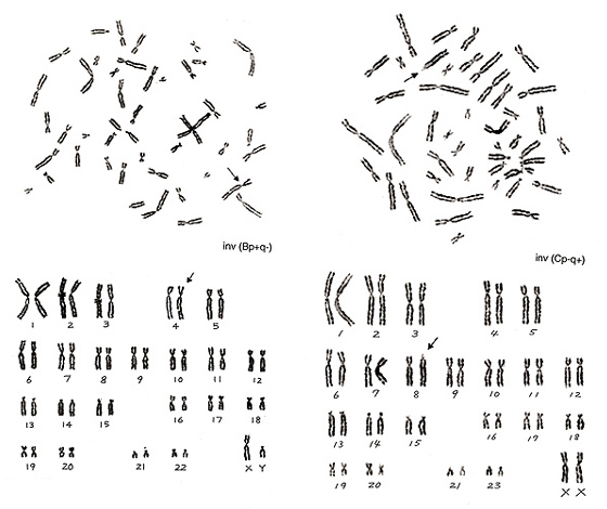
Figure 14
The inversion on the right panel resulted in a monster of a group-D or -G chromosome. After understanding that the total length of this abnormal chromosome is within a group-C chromosome and that the number of group-D and group-G chromosomes is normal (six and four, respectively), identification of inversion is not difficult.
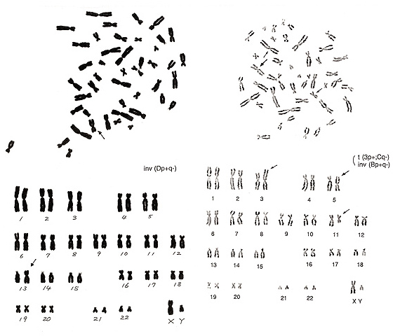
Figure 15
The metaphase of Figure 15 (left) contains five group-G chromosomes (one of these is a Y chromosome), 16 group-C chromosomes (normally 15 as the donor is a male), and five group-D chromosomes (normally six). The additional group-C chromosome appears to be a small chromosome, and the length does not differ from a group-D chromosome. Thus, it seems likely that one group-D chromosome underwent an inversion and that the centromere position became near the center of the chromosome, a characteristic of group-C chromosomes. It may be problematical that one chromosome is located far away from the remaining chromosomes in the metaphase figure. Unless complete karyotyping is performed, this cell might indicate a numerical abnormality.
The metaphase shown in Figure 15 (right) is more complicated. It indicates an inversion of a group-B chromosome, which resembles a normal chromosome 3 (arrowed chromosome 5 in the lower panel). This is classified as an inversion because the inverted chromosome has slightly shorter p and q arms than a normal chromosome 3. Another aberration is present in this metaphase. Specifically, one chromosome is similar to a normal chromosome 1 but has no “h” (arrowed chromosome 3), and one chromosome is similar to a normal chromosome 16 but has a shorter p arm (arrowed chromosome 11). Thus, it is possible to interpret the aberration as t(Bq-; Cp+) without inversion of a group-B chromosome, i.e., take the marked chromosome 5 as a normal chromosome 3. However, I felt it difficult to regard the arrowed chromosome 5 as a normal chromosome 3 because of the different length, and preferred to consider the metaphase to contain two aberrations, one inversion and one translocation.
10. Stable aberrations – reciprocal translocation
Reciprocal translocation is the most predominant type of stable aberration, comprising nearly 70% of the total stable aberrations in lymphocytes from the atomic-bomb survivors. As radiation exposure randomly breaks DNA, the induction rate of translocation is roughly proportional to chromosome length.
There are various difficulties in detecting translocations by the conventional method. For example, when the two chromosomal segments that underwent exchanges are similar in length, such exchanges can never be detected. Furthermore, translocations between group-C chromosomes that are similar in length and shape are detected much less frequently. This is the limit of detecting stable aberrations by the conventional method.
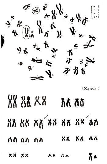
Figure 16
The metaphase presented in Figure 16 (top) shows no abnormalities in chromosomes of groups A, D, F, G, and Y, but there are five group-B chromosomes (gain of one chromosome) and three number 16-like chromosomes (gain of one chromosome) along with 13 group-C chromosomes (deficit of two chromosomes as the donor is a male). Karyotyping results (Figure 16 [lower]) clarified that one group-C chromosome has an extended long arm, resulting in a shape similar to a group-B chromosome, and another group-C chromosome underwent shortening of its long arm, resulting in a chromosome similar to a normal chromosome 16. In other words, a reciprocal translocation between the two group-C chromosomes resulted in creating one group-B-like and one chromosome-16-like chromosome. Thus, the aberration was assigned as t(Cq+; Cq-).
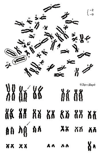
Figure 17
The metaphase shown in Figure 17 includes one group-D chromosome with its extended long arm, missing one chromosome 2, and one number 17-like chromosome with its abnormally extended long arm. Karyotyping results show a translocation between the chromosome-2 short arm and group-D chromosome long arm, or t(2p-; Dq+) (Figure 17 [lower]).
The following several figures show translocations involving the longest chromosome 1. The chromosomes that underwent translocations are marked by the arrows.
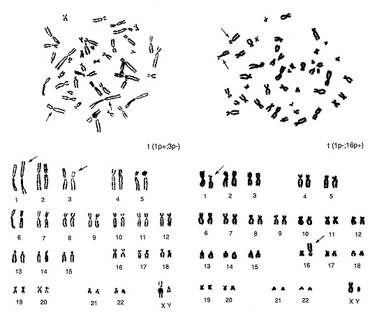
Figure 18
The metaphase shown in Figure 18 (left) contains several overlapped chromosomes, and the chromosomes are thin. Thus, karyotyping may be difficult for beginners. The abnormalities are seen in one group-A chromosome (lack of one chromosome 3) and in one group-C chromosome (additional chromosome). It also shows one of the two chromosome 1s has both arms longer than usual. When we look at this chromosome carefully, the “h” of the abnormal chromosome 1 is abnormally long, but this is a normal variant. As this is a normal variation, the actual abnormality exists on its short arm. If we consider that the additional apparent group-C chromosome is derived from one chromosome 3, the aberration is interpreted as t(1p+; 3p-).
In Figure 18 (right), chromosome 1p (short arm) is shorter, and a large “h” is seen near the centromere. At the same time, we see that one of the group-E chromosomes (chromosome 16) is missing and one additional group-B chromosome is present. Consequently, the translocation seems to have occurred between chromosome 1p and chromosome 16p or t(1p-; 16p+). The two metaphases in Figure 18 are from the same individual, and thus the same normal variation of “h” in chromosome 1 is observed in the two figures.
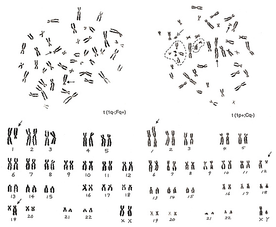
Figure 19
The metaphase in Figure 19 (left) has lost one chromosome 1 and one group-F chromosome, but has two additional group-C-like chromosomes. Thus, the aberration is t(1q-; Fq+).
The metaphase in Figure 19 (right) contains one chromosome 1 with its short arm extended (arrowed chromosome 1) and six group-G chromosomes (one of them is a Y chromosome), and one group-C chromosome is missing. Thus, we suspect that the extra group-G-like chromosome is derived from one group-C chromosome whose long arm was mostly moved to the short arm of chromosome 1, or t(1p+; Cq-). Which of the five apparent group-G chromosomes is involved in the aberration? We see that four out of the five chromosomes, excluding the Y chromosome (marked with a broken arrow), are in the dotted circle that is the satellite association (“sa”). Normally, both group-D and -G chromosomes participate in the “sa” formation. Thus, these four chromosomes are true group-G chromosomes, and the remaining one (arrowed chromosome 12) is deduced as the aberrant group-C chromosome.
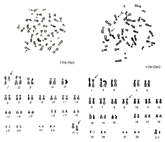
Figure 20
The metaphases shown in Figure 20 also represent translocations involving chromosome 1. The left figure shows that one chromosome 1 is missing and that there is one big group-D-like chromosome (arrowed Y chromosome in the lower figure). We know that the lower half of a Y chromosome long arm usually comprises an “h” and that this segment tends to be more closely associated than group-G chromosome arms. The upper half of this aberrant group-D-like chromosome bears a characteristic of the Y-chromosome long arm. It thus seems likely that the majority of the chromosome-1 long arm was transferred to the Y chromosome, namely, t(1q-; Yq+).
The metaphase of Figure 20 right contains several abnormalities. The short arm of chromosome 1 became shorter, and the “h” of this chromosome is quite large. The translocation partner is one of the group-C chromosomes with a large “h”, probably chromosome 9, and the long arm became longer. Thus, the aberration is interpreted as t(1p-; Cq+).
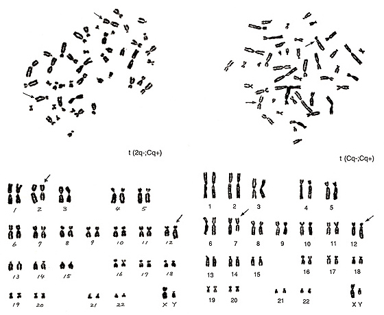
Figure 21
The metaphase of Figure 21 (left) contains three number 3 chromosomes and one extra group-B chromosome. If you could recognize these two strange chromosomes without karyotyping, you are no longer a novice. The following characterization is rather straightforward, and the aberration can be interpreted as t(2q-; Cq+).
The metaphase of Figure 21 (right) represents the most difficult translocation between two group-C chromosomes. The abnormal chromosomes indicated by arrows suggest that one is a small chromosome with a centromere located close to the middle, and the other looks like a group-B chromosome but with a small short arm. Among the several possibilities, t(Cq-; Cp+) seems to be a reasonable interpretation.
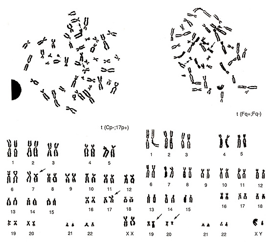
Figure 22
The two metaphases shown in Figure 22 represent examples of translocations involving small chromosomes. The abnormality in the left figure would be difficult to detect by simple observation of the metaphase. If you examine it carefully, however, you may find that one group-E chromosome, probably chromosome 17, is missing and one extra group-C chromosome is present. As the smaller group-C-like chromosome has its centromere near the middle of the chromosome, it must be an aberrant chromosome. Instead, the middle-sized group-C-like chromosome has a strange CI (p arm is too short and q arm is too long), and it is important to consider that it does not appear to be a normal group-C chromosome. Thus, the karyotype suggests t(Cp-; 17p+) as the most reasonable explanation.
The metaphase shown in Figure 22 (right) has two missing group-F chromosomes. One chromosome is similar to chromosome 16 or 17, but neither of these are likely, and one chromosome is smaller than the group-G chromosome. This is suggested to be due to a translocation between two group-F chromosomes, t(Fq+; Fq-).
As you see from the last example, translocations involving small chromosomes like groups F and G can be detected with relative ease, even though the gain or loss of the chromosome segment may be small. Thus, detection of stable aberrations by the conventional method tends to under score the aberrations in large chromosomes.
11. Example of misinterpretation
Here I will show you one example of misinterpretation. The metaphase shown in Figure 23 (left) is a representative normal karyotype. It is the same as shown in Figure 6 (left), and its proper karyotype is shown on the right upper panel.
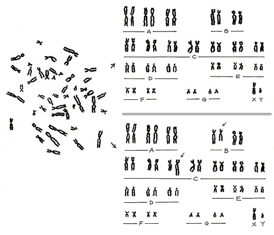
Figure 23
However, if a misinterpretation is made, an abnormal pattern is created as an artifact (right lower panel). In other words, a normal karyotype can become abnormal if we misalign two normal chromosomes. Experience will certainly reduce such errors, but the pitfall will always remain. If you suspect an aberration, it is important to take a photograph as proof.
12. Conclusions
Yukichi Fukuzawa is known as the founder of Keio University and is famous for his expression, “God did not make people above or below others.” He contributed significantly to the modernization of the Japanese educational system when Japan decided to open the country to foreign countries at the time of the Meiji revolution. He stated the following in his book titled “Current medical methods.”
“I believe that to be healthy is common and to be ill is abnormal, but without knowing the common, we cannot know the abnormal.” This sentence is quite reasonable. If we interpret “common” as “normal chromosomes” and “illness” as “abnormal chromosomes,” we may state that “How can we understand chromosome aberrations without knowing normal chromosomes?” I feel that his statement can be applied to scientists in general in the sense that we need to know the normal to understand the abnormal.
Such an attitude is not restricted to Yukichi Fukuzawa. While reviewing his life, a famous American golfer said, “To do a good job, it would suffice to repeat subtle but fundamental works.”
The fundamental works are nothing special. They are simple, clear, and not difficult to learn. However, as usual, it is easy to say but more difficult to do.
As I repeatedly stated in this manual, even though there are many different types of chromosome aberrations, there is only one normal pattern. Thus, without knowing the normal, we cannot understand the abnormal. It is unfortunate, but there is no shortcut to learning the normal, just some key information. Basic understanding is important in any field but it requires patience. Nonetheless, there is hope because we now know that it is possible to achieve it.
To close the manual, I would like to describe a short history about how the correct number of human chromosomes was derived. In 1956, Drs. J. H. Tjio and A. Levan were the first to report that the number was 46. I was a master’s course student at that time and was shocked to find that the 47 and 48 theories were wrong.
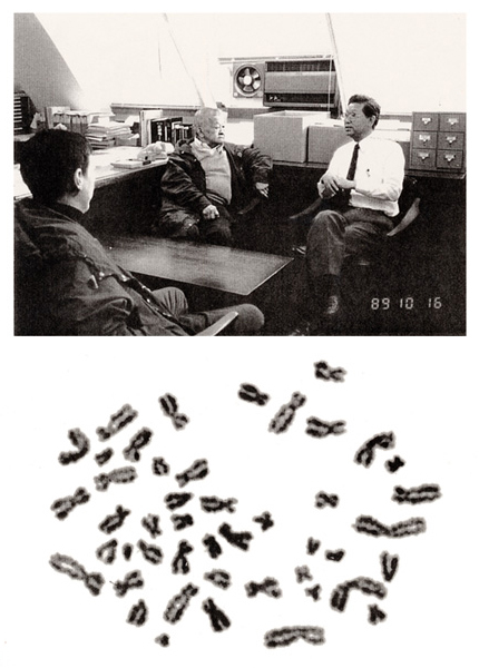
Figure 24
In October of 1989, Dr. Tjio and his family visited RERF. He worked at the National Institutes of Health in the United States, and I heard a rumor that he was a difficult person. In fact, however, he was not. After his return to the USA, I received his mail including two photographs.
Here, I show his picture (at middle, top panel) and his metaphase used in the 1956 Hereditas paper at the end of this manual.